![]()
Despace tutorial and examples
Installation
[ ]:
!pip install despace --upgrade
Usage
[2]:
from despace import SortND
import numpy as np  # for generating random data
Use cases
SortND is a python class for sorting N-D array-like data and visualize the sorted data if the number of dimensions is <=3.
1. Sort 2D coordinates
[3]:
data = np.random.rand(100, 2) # Let's generate some random data
We can either initiate the SortND class with data and then use the sort method, or initiate the SorND class withtou providing data, but then directly call with data.
[4]:
s = SortND(data)
s.sort()
s.plot(show_plot=True, plot_arrow=True)

[4]:
True
The data is colored from blue to red as the index goes higher. The arrows coonect two successive data points.
If we don’t want the arrows that show the relative indices in the sorted data, we can set plot_arrow to False
[5]:
s.plot(show_plot=True, plot_arrow=False)

[5]:
True
Let’s look at the sorted data:
[6]:
s.sorted_coords[0:20,:]
[6]:
array([[1.20941257e-01, 5.91526257e-02],
       [3.25718514e-02, 9.74565620e-02],
       [1.62132588e-01, 1.35027698e-01],
       [3.25022682e-01, 7.93149650e-03],
       [1.75661503e-01, 7.94614740e-02],
       [2.07350441e-01, 1.59170200e-01],
       [2.38184967e-01, 2.97525569e-01],
       [7.02506519e-03, 3.43268630e-01],
       [1.73103492e-02, 3.49722952e-01],
       [3.19409889e-01, 2.07180786e-01],
       [2.70387646e-01, 4.61570909e-01],
       [2.73479793e-01, 4.65325404e-01],
       [3.74223225e-01, 1.43901996e-02],
       [3.44131364e-01, 1.17916049e-01],
       [3.61386002e-01, 6.23778659e-02],
       [4.16027140e-01, 1.15405545e-06],
       [4.42175562e-01, 2.49551881e-02],
       [4.55579364e-01, 1.82072067e-01],
       [4.17344346e-01, 2.39805423e-01],
       [3.46449546e-01, 4.55420742e-01]])
2. Sort 3D coordinates
[7]:
data = np.random.rand(1000, 3)
s(data)
s.plot(show_plot=True)

[7]:
True
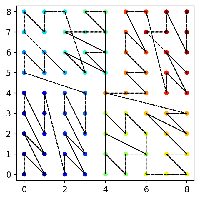
3. Space filling curves
Morton space filling curve
[8]:
data = [[i, j] for i in range(8) for j in range(8)]
s.sort(data)
s.plot(show_plot=True, plot_arrow=True)

[8]:
True
If one dimension length is odd:
[9]:
data = [[i, j] for i in range(8) for j in range(9)]
s.sort(data)
s.plot(show_plot=True, plot_arrow=True)

[9]:
True
The path can cross itself in the ‘odd’ dimension.
If both dimension lengths are odd:
[10]:
data = [[i, j] for i in range(9) for j in range(9)]
s.sort(data)
s.plot(show_plot=True, plot_arrow=True)
[10]:
True
Since the order is random if two points have the same value in either of their components, we see move data cross-over in both directions!
Hilbert space filling curve (2D)
If we set sort_type='Hilbert':
[11]:
data = [[i, j] for i in range(16) for j in range(16)]
s.sort(data, sort_type='Hilbert')
s.plot(show_plot=True, plot_arrow=True)
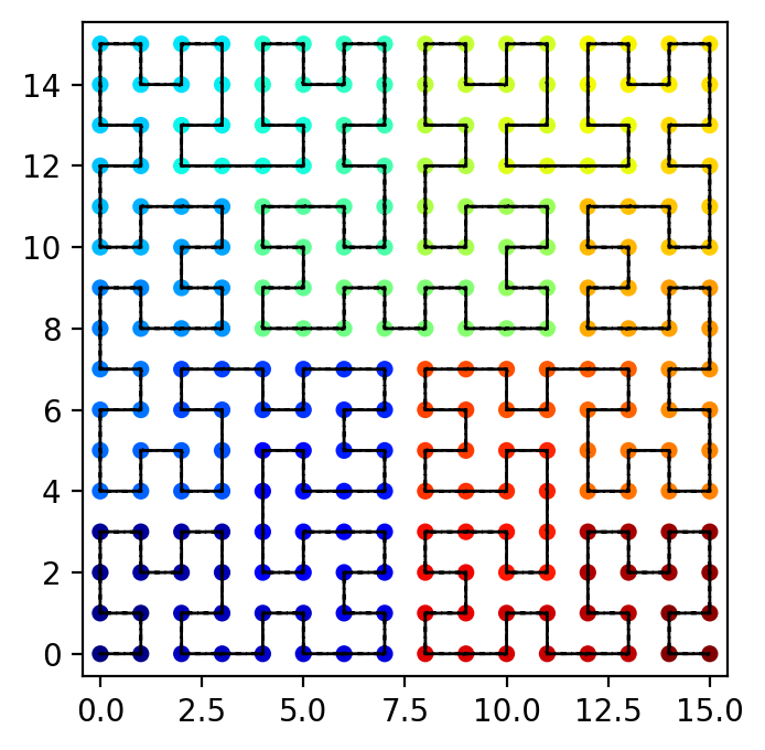
[11]:
True